The Production Function

Inputs and Outputs

To produce anything, firms must have inputs and outputs. The firm's inputs are the resources that the firm needs to produce the outputs, or the products that the firm sells. For example, a pizza restaurant need flour, cheese, pepperoni, and sauce to make pizzas. These resources are the pizza restaurant's inputs. Since the pizza restaurant produces pizzas, the pizzas are the firm's outputs. The number of workers employed by the firm is another example of an input.

Input resources are also called factors of the firm.

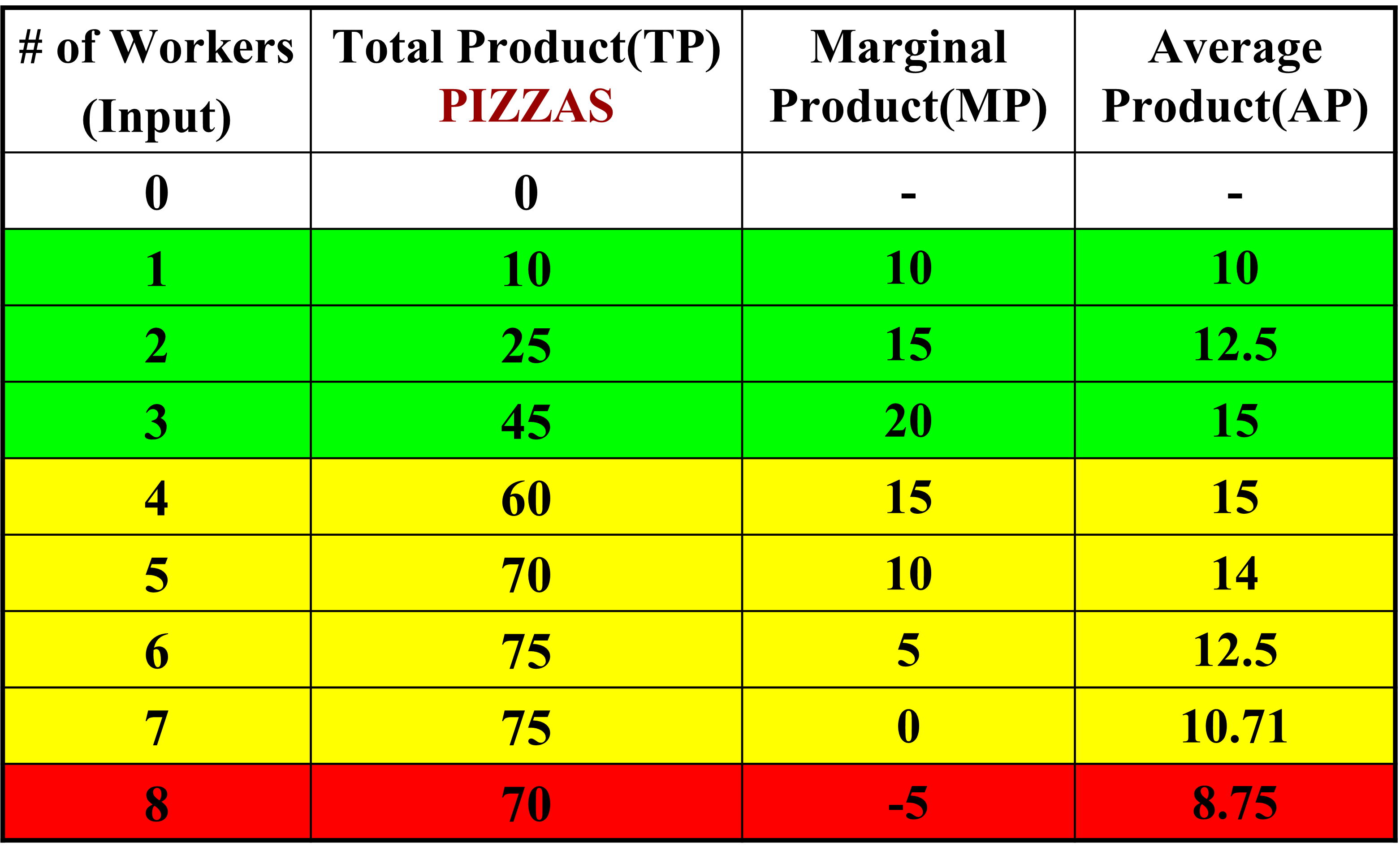
Total Physical Product (TP) is the total output/total quantity that the firm produces.

Marginal Product (MP) is the additional product that can be produced for every additional input provided.

$$\text{Marginal Product} = \frac{\Delta \text{TP}}{\Delta \text{Input}}$$

Average Product is the total output per unit of labor.

$$\text{Average Product}=\frac{\text{TP}}{\text{Total Input}}$$

Types of Resources

There are two major types of resources:

• Fixed Resources - Resources that remain constant regardless of the quantity of product produced
• Variable Resources - Resources that change based on the quantity of product produced

If we return to our pizza restaurant example, fixed resources would be the cost of a pizza oven, as the cost of the oven does not change if more pizzas are produced. A variable resource would be cheese. More cheese must be purchased as the quantity of pizzas produced increases (or else the restaurant will run out of cheese for its pizzas).

Production Analysis

Assume there is 1 worker at the pizza restaurant when it opens. This worker must put the pizza in the oven, wait for it to come out, take the pizza to the topping center, put the toppings on the pizza, add the sauce and cheese, and then box the pizza and deliver it. This process will take a very long time, and few pizzas will be produced per day. As the number of workers increases to 2 or 3, workers can begin to create an 'assembly line'. One worker will man the oven, another worker will add the toppings, and yet another will box the pizzas. This process is called specialization, as each worker becomes efficient at one specific task.

But what happens when you hire even more employees, let's say 20 or 30 more employees. The restaurant starts to become crowded and the manager begins to have a hard time keeping track of what each worker is doing. Some workers aren't doing any work because all the ovens are already being watched and the pizzas are coming out too slow compared to the number of workers. This means that the restaurant becomes less efficient, reducing the marginal product! This establishes a rule in economics:

The Law of Diminishing Marginal Returns - As variable resources are continually added to fixed resources, the additional product produced by each worker eventually begins to decrease.

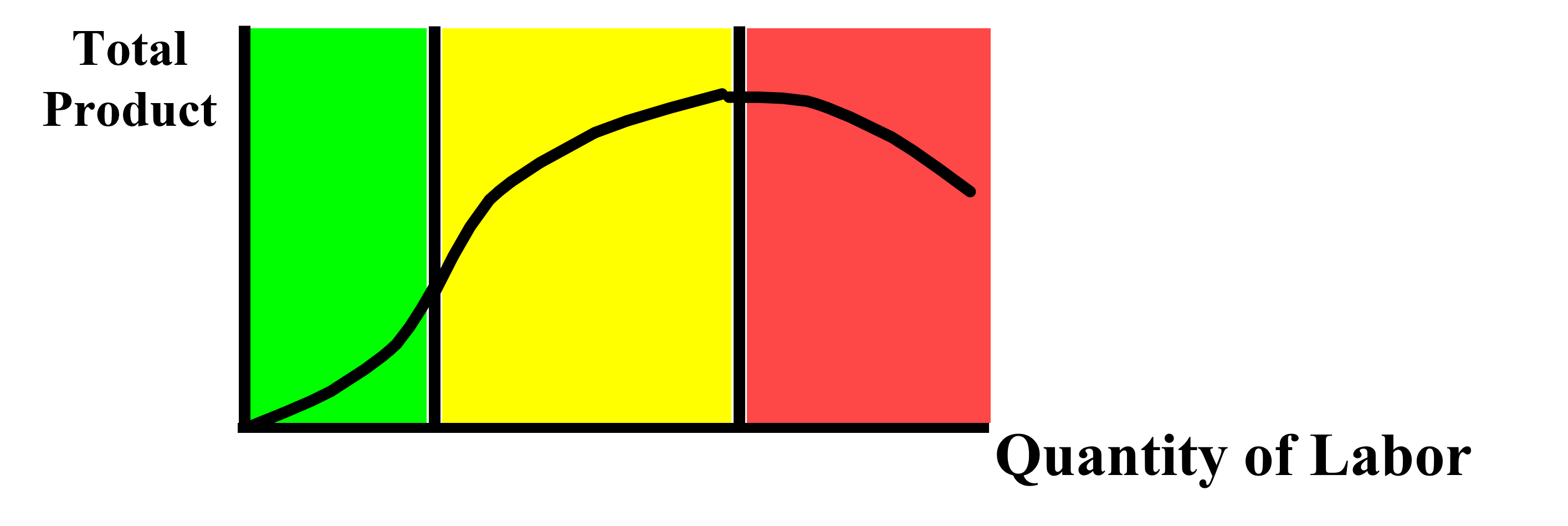
Graphing Production

There are three stages of the output produced by a firm:

1. Increasing Marginal Returns \(\rightarrow\) Total product increases faster
2. Decreasing Marginal Returns \(\rightarrow\) Total product increases slower; total product curve eventually levels out
3. Negative Marginal Returns \(\rightarrow\) Total Product decreases faster and faster

Production Costs

In economics, two terms are commonly referred to: the short run and the long run. Contrary to their names, the short run and long run are not specified lengths of time.

In the short run, at least one resource cannot be changed, and in the long run, all resources can be changed, and all resources are variable. For example, in the short run, a firm cannot easily purchase another factory if they need more space for production, but when they expand, they have enough profit that they can quickly make the decision if another factory is necessary.

Now we can define the various types of economic costs:

Total Costs

• FC - Total Fixed Cost
  • Costs that don't change based on the quantity of product produced
  • Ex: Rent, Salary, Insurance
• VC - Total Variable Cost
  • Costs that do change based on the quantity of product produced
  • Ex: Raw Resources, Workers/Labor, Electricity, Water
• TC - Total Cost
  • The sum of fixed cost and variable cost
  • \(\text{TC} = \text{FC} + \text{VC}\)

Per Unit Costs

• AFC - Average Fixed Cost
  • \(\text{AFC} = \frac{\text{Fixed Cost}}{\text{Quantity}}\)
• AVC - Average Variable Cost
  • \(\text{AVC} = \frac{\text{Variable Cost}}{\text{Quantity}}\)
• ATC - Average Total Cost
  • \(\text{ATC} = \frac{\text{Total Cost}}{\text{Quantity}}\)
• MC - Marginal Cost
  • Additional cost of making another item
  • \(\text{MC} = \frac{\Delta \text{Total Cost}}{\Delta \text{Quantity}}\)

Another important property of costs is that \(\text{ATC} = \text{AFC} + \text{AVC}\), which can be observed in the table below.

As you can see in the table, the fixed cost remains the same as the output changes, while the variable cost increases as output increases. In other words, only the first output item receives the fixed cost.

Now we graph the curve corresponding to these costs:

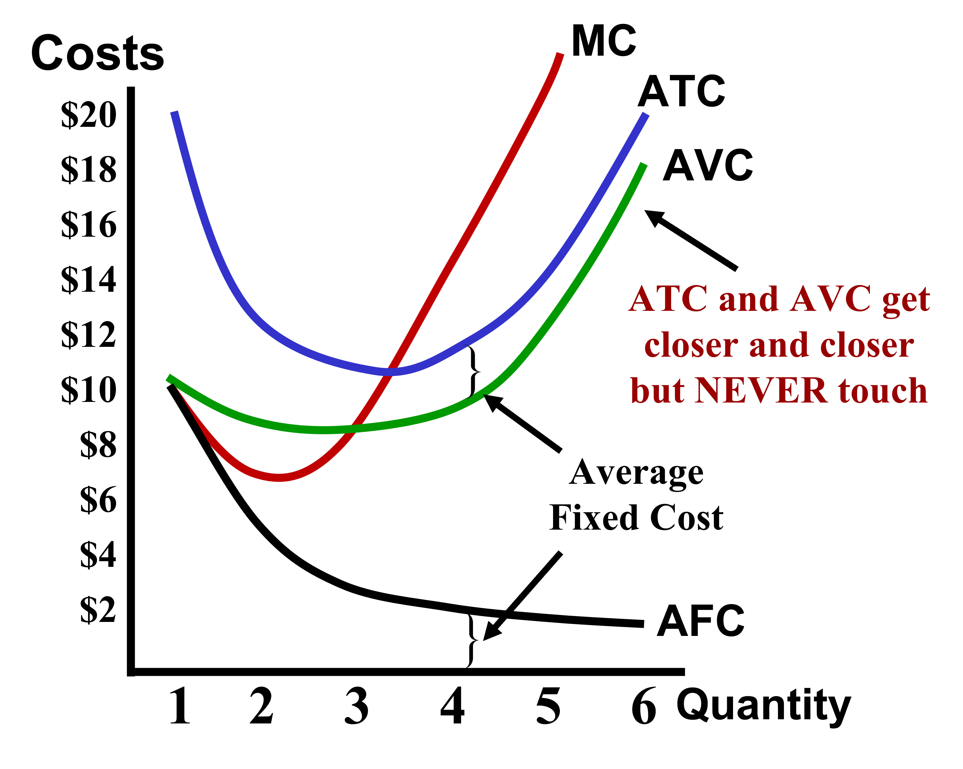
This graph must be memorized, and an easy way to do this is to remember that the Marginal Cost curve looks like Nike's swoosh logo, and ATC is basically AVC but shifted upward by a small amount.

Two important thing to keep in mind are that the AFC decreases as quantity increases, but never reaches \(0\). Since \(\text{ATC} = \text{AFC} + \text{AVC}\) and \(\lim_{Q\to\infty} \text{AFC} = 0\), \(\lim_{Q\to\infty} \text{ATC} = 0 + \text{AVC} = \text{AVC}\).

Another important thing to remember is that the MC curve intersects the ATC curve at the ATC's minimum point. One way to conceptualize why this occurs is by thinking of grades. Assume the ATC curve is your end-of-year grade and the MC curve is the individual grade you get on each assignment. As long as the grade you get on your next assignment is above your average, your average grade will increase. If you get a score lower than your average, your average will decrease. In other words, the MC has the ability to either pull the ATC up or down based on its relationship to the ATC curve.

Economies of Scale

Firms can expand their production by purchasing more resources, hiring more workers, and making their technology better. But is expanding worth it if the company makes the same profit relative to their size? This where economies of scale come into the picture.

There are three types of economies of scale:

1. Increasing Returns to Scale \(\rightarrow\) Output more than doubles when inputs are doubled
2. Constant Returns to Scale \(\rightarrow\) Output doubles when inputs are doubled
3. Negative Marginal Returns \(\rightarrow\) Output less than doubles when inputs are doubled. This is also called diseconomies of scale

In each of these cases, returns refer to the firm's production, not the firm's costs.

Economies of scale can occur because mass production reduces average costs. For example, producing one car can cost hundreds of thousands of dollars, but car companies reduce their prices by purchasing resources in bulk and mass producing cars. The total cost of making all the cars is much higher than making one car, but since so many are being produced, the average cost of each car is significantly lower.

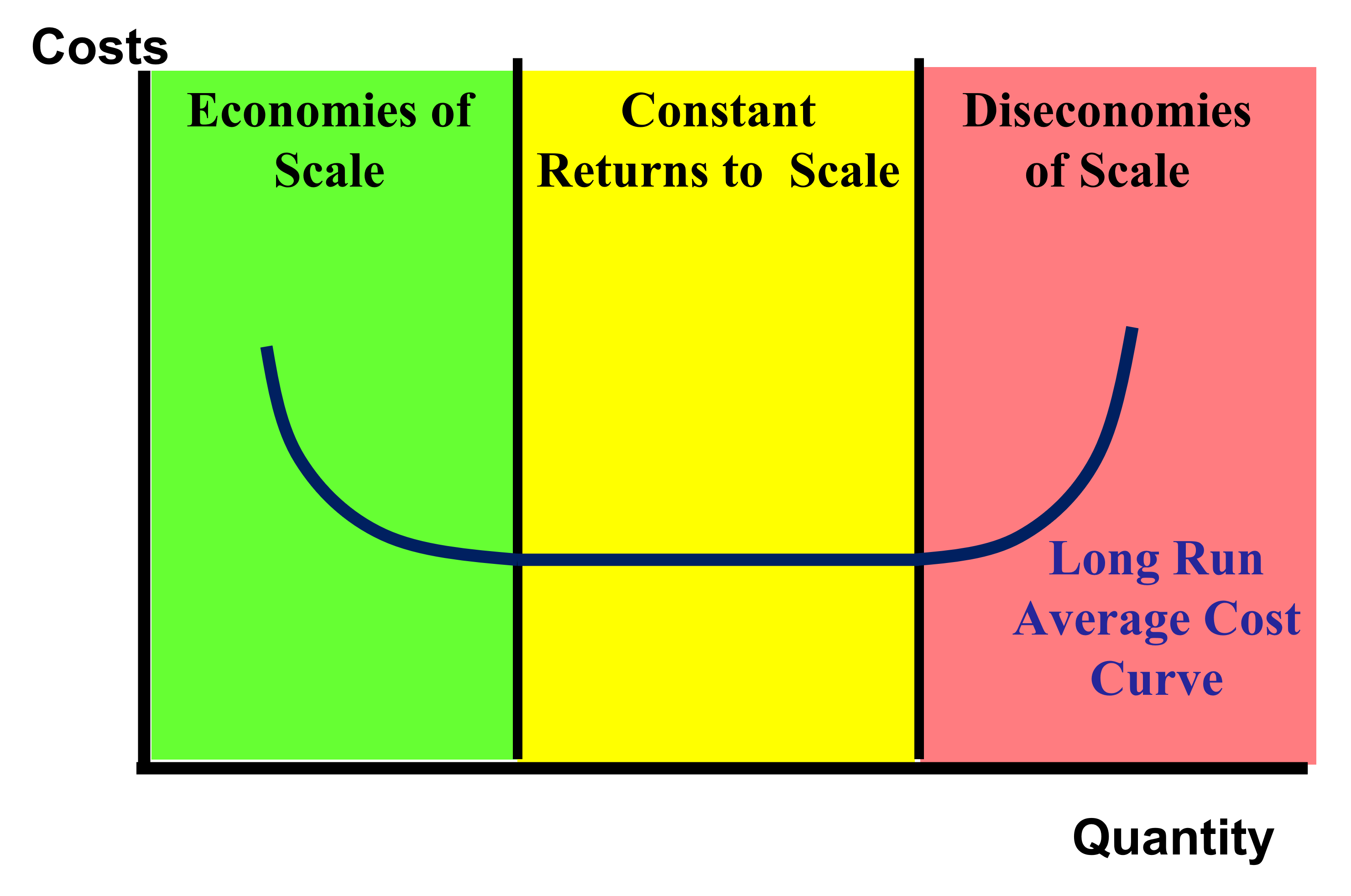
Long Run Average Total Cost

The long run average total cost curve is made up of all the points of intersection of the short run ATC and MC curves of the company. An example of a long run average total cost curve is shown below. Each of the intersections of MC and ATC corresponds to a different scale of the car firm we are examining.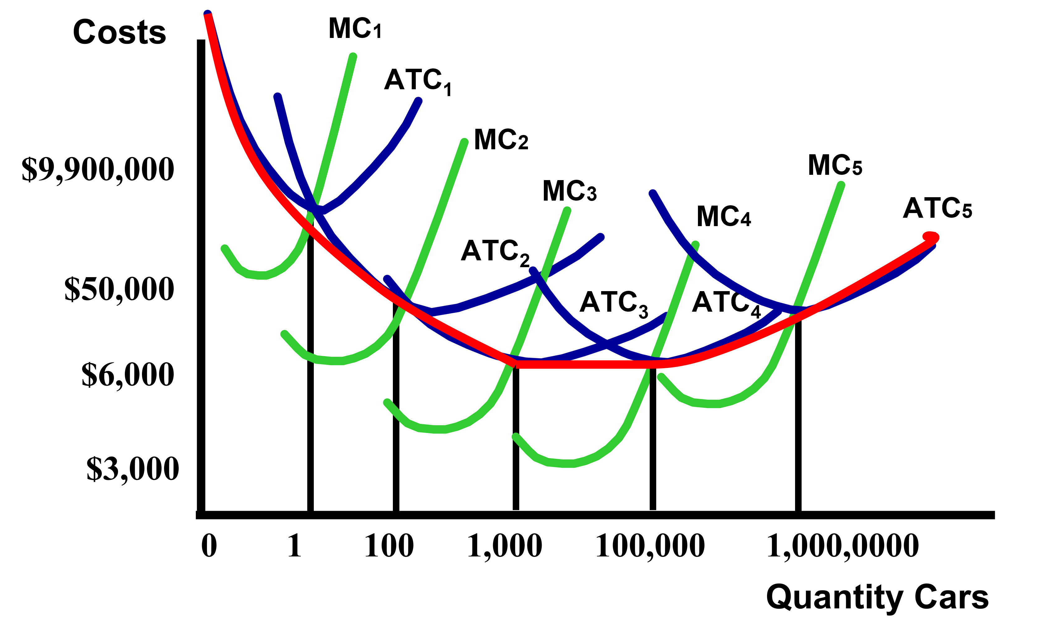

Now we can also identify the parts of the curve that correspond to the three stages of an economy of scale: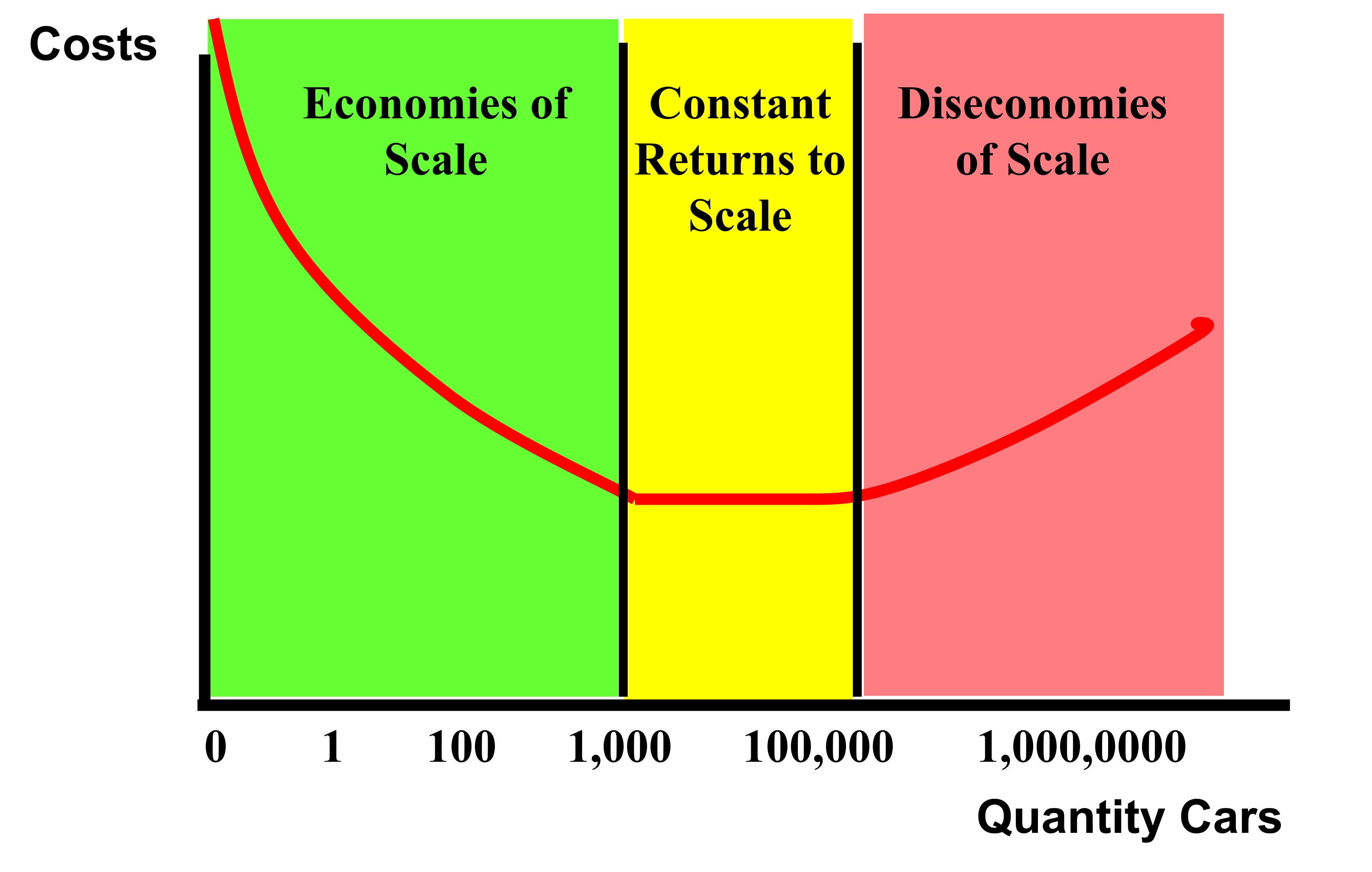

We can also simplify the long run average total cost curve by graphing cost vs quantity:

Types of Profit

We already know the formula for total revenue:$$\text{TR} = \text{Price} \times \text{Quantity}$$

Now we define the formula for a firm's profit:$$\text{Profit} = \text{Total Revenue} - \text{Total Cost}$$

There are two different types of profit:

• Accounting Profit - Monetary profit. Only money costs and money revenue is taken into account.
• Economic Profit - Both explicit and implicit costs are taken into account. Unlike accounting profit, economic profit also includes opportunity costs such as forgone wage, forgone rent, and time.

This means that accounting costs are the monetary explicit costs while economic profit is the explicit monetary costs along with the implicit opportunity costs.

Since economic profit includes more costs than the accounting profit, we know that \(\text{Economic Profit} \le \text{Accounting Profit}\) is always true. When there is no economic profit, we call the profit a normal profit.

In economics, the word 'profit' always mean economic profit unless specified by the question.

Profit Maximization

The goal of every firm is to maximize their profit, but how do they know what quantity to produce at? To find this profit-maximizing output, the firm can use their cost curves.

Firms should continue to produce as long as their marginal revenue for the new output is greater than or equal to their marginal cost. Therefore, to find the profit maximizing output, the firm must find where the \(\text{MR}=\text{MC}\).

Decisions to Enter or Exit the Market

Firms have to constantly analyze their profits and losses to determine whether they should shut down or continue to produce. Although this decision might seem simple - shut down when making a loss and continue to produce when making a profit - this is not completely correct. Here is the correct rule:

Firms should continue to produce as long as their Average Variable Cost curve is below the price. As long as the AVC is less than profit, the firm is making enough money to pay off all the average variable cost as well as part of the fixed cost they paid when entering the market. In this way, the firm is minimizing their losses even though they are not making a profit.

The following image shows the cost curves for a firm. As long as the selling price of the firm's product is above \($5\), the firm should continue to produce. When the price falls below this point, the firm must shut down.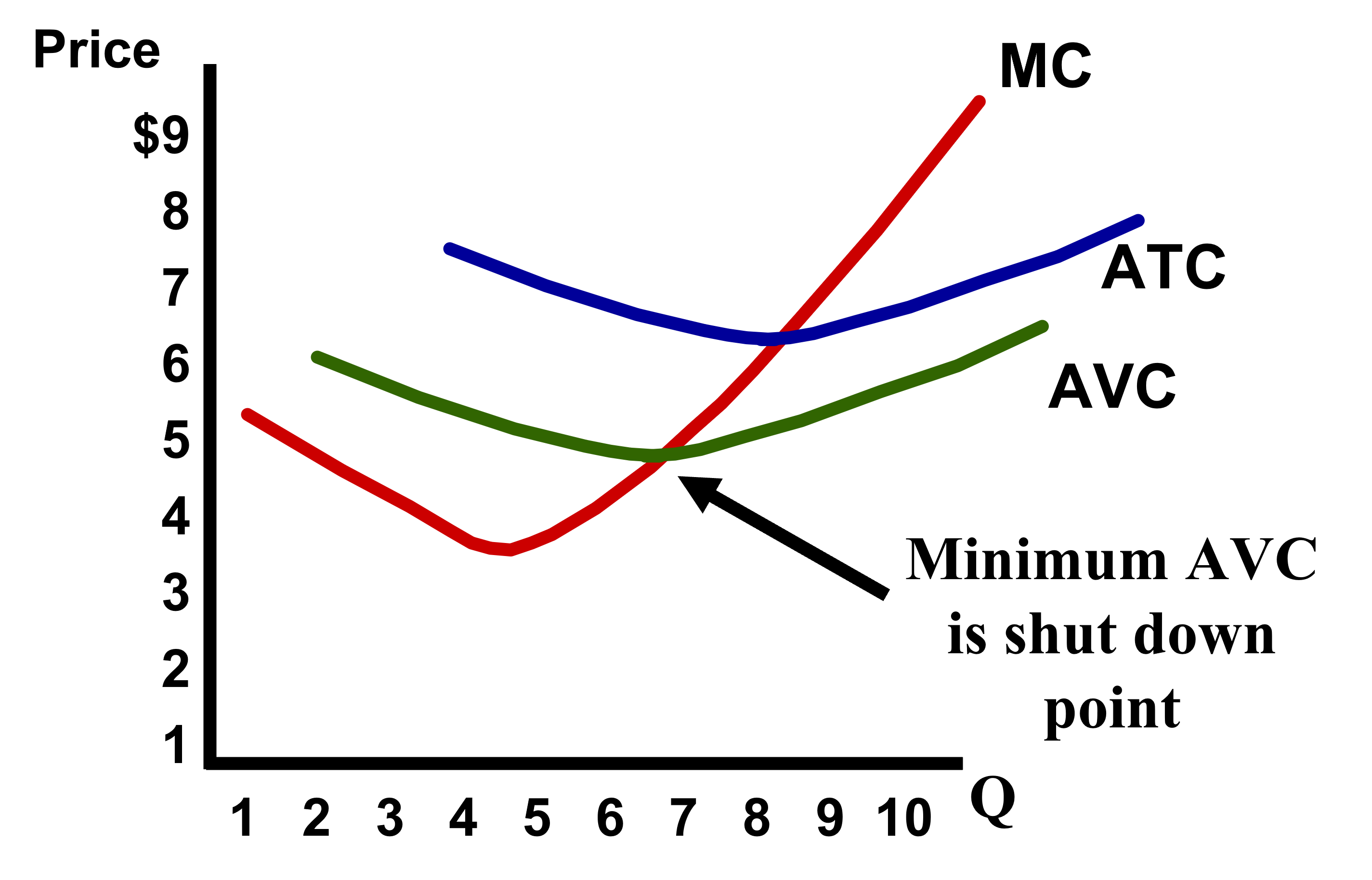

Another important thing to remember is that the MC curve above the minimum AVC is the short-run supply curve.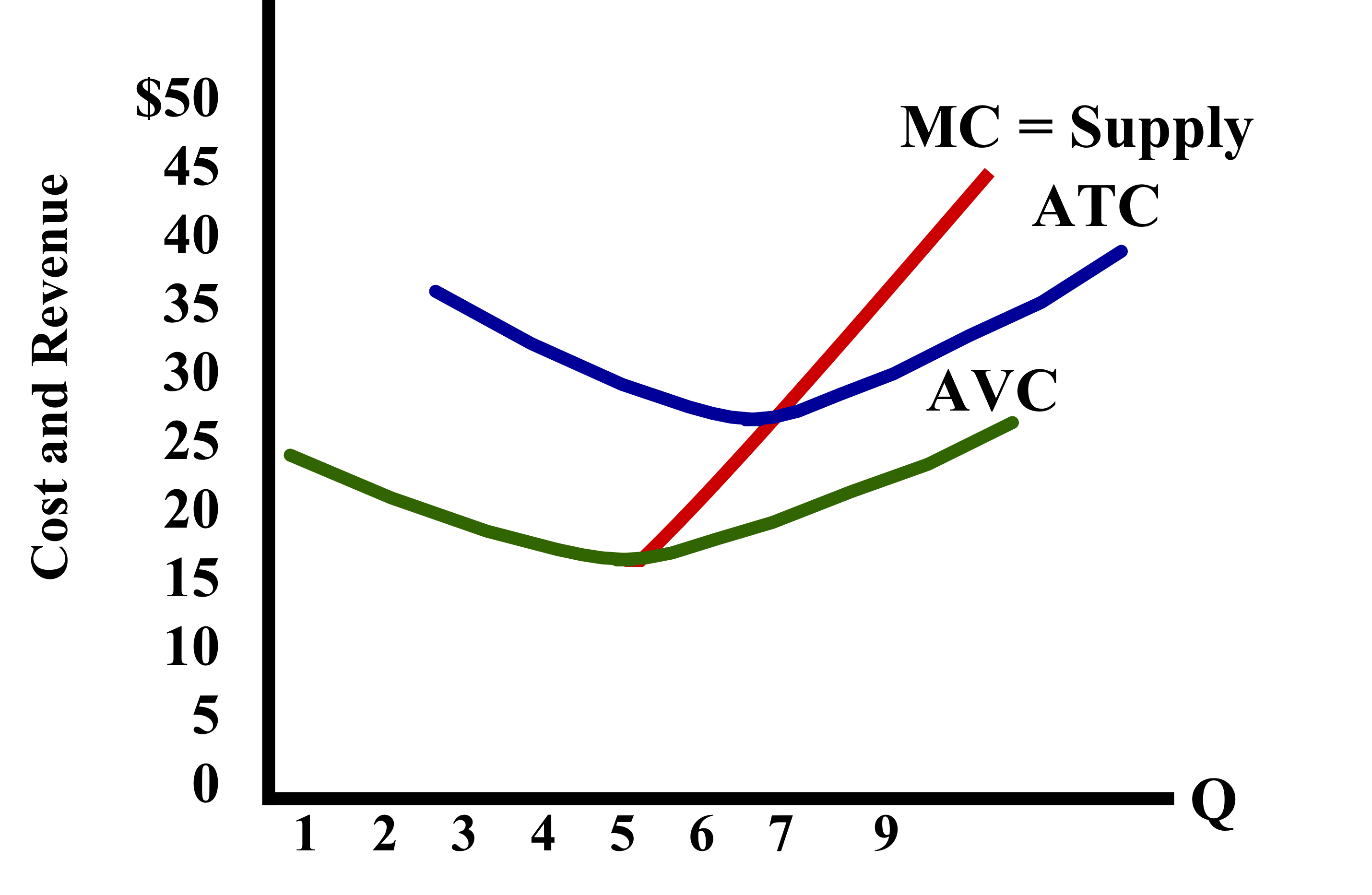

Now that we've analyzed what firms do in the short run, we need to see what firms do in the long-run.

In the long run, other firms enter the market if a firm already in the market is making a profit. If the firms already in the market are making a loss, those firms will exit the market.

Firms continuously entering and leaving the market lead to an eventual equilibrium point, where all firms in the market are making neither a profit nor a loss. Remember that the profit we are referring to is economic profit, which means that the firms in the market are still making an accounting profit and still earning money! Normal Profit = No Economic Profit = Positive Accounting Profit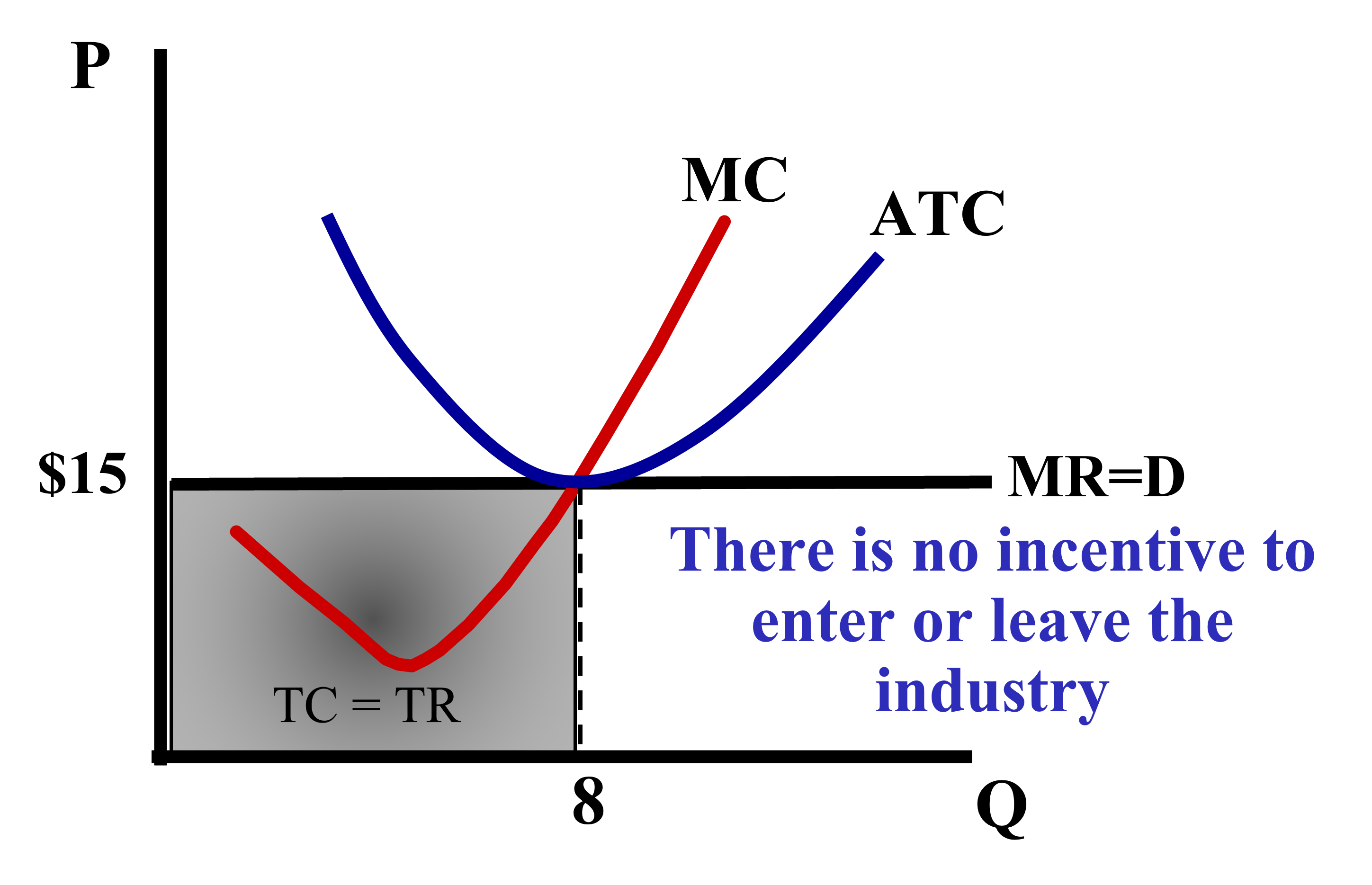

Barriers to Entry

Barriers to entry are the factors that prevent firms from entering into a market.

If a market has high barriers to entry, firms in the market have low competition and each firm makes more profit. An example of such a market is the airplane/flight market. To enter this market, a company must first purchase planes, purchase space at airports, and then convince customers that their flights are better than the other already established companies.

If a market has low barriers to entry, firms in the market have high competition and each firm does not make much profit. An example of market with low barriers to entry is the agriculturual market. Anyone who has a backyard can enter the agriculture market by planting some seeds and watering them.

When a market is in perfect competition, firms have low barriers to entry.

Perfect Competition

The following are characteristics of a market with perfect competition:

• Many small firms
• Identical products/perfect substitutes
• Low barriers to entry
• Firms have no control over the price - demand leads to changes in price.

In perfect competition, firms must adapt their prices to reflect consumers' demand. If the firm charges a price higher than what consumers want to pay (the market price), consumers will stop purchasing from that firm and simply buy from another since all products of that type are identical.

This means that the demand curve in perfect competition is perfectly elastic and a horizontal line.

The graph for perfect competition can be drawn as shown below: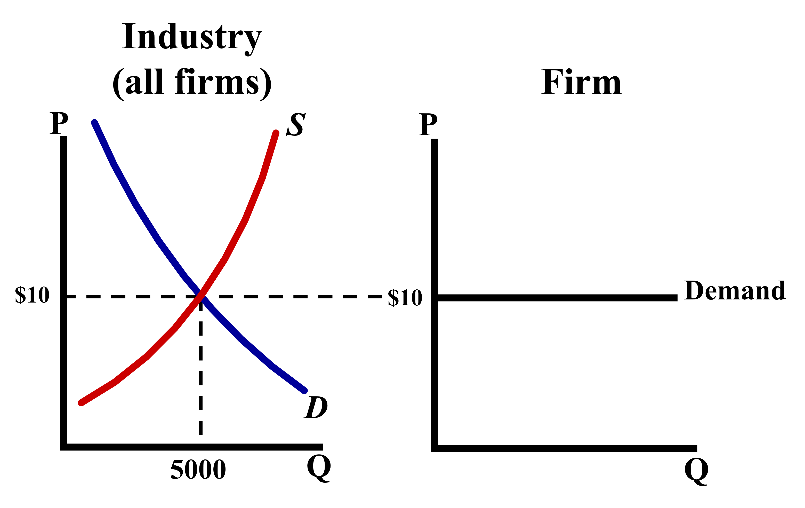

An important thing to keep in mind when graphing perfect competition is that \(\text{Marginal Revenue} = \text{Demand} = \text{Average Revenue} = \text{Price}\). This can be remembered by thinking about the acronym 'Mr. Darp' (\(\text{MR} = \text{D} = \text{AR} = \text{P}\)).

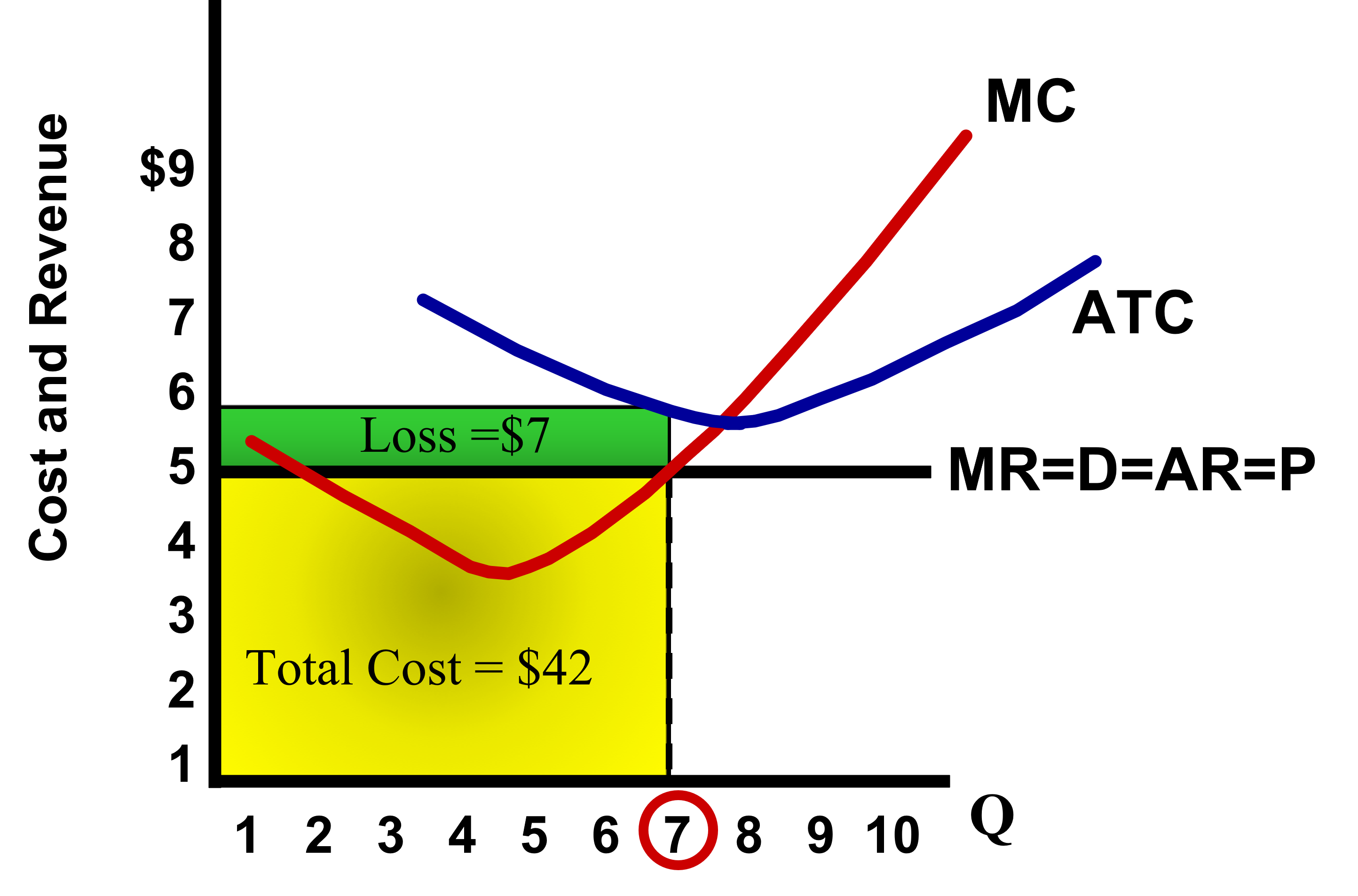
Although these graphs might look confusing, the fundamental rules of economics still remain true. Profit is still maximized when the marginal revenue equals the marginal price.

We still have \(3\) basic steps to find the profit or loss on the graph:

1. Find the profit maximizing point by finding where \(\text{MR} = \text{MC}\).
2. Draw a vertical line touching the ATC curve to find the total cost incurred.
3. Calculate the profit through the formula \(\text{Profit} = \text{Quantity} \times (\text{MR} - \text{ATC})\).

A diagram of this process for a firm with a loss is shown below:

Shifting Cost Curves

All you need to know about shifting cost curves is the following two facts:

• Changes in fixed costs changes the ATC and AFC curves, but not the MC curve
• Changes in variable costs changes the ATC, AVC, and MC curves, but not the AFC curve

Perfect Competition in the Long Run and Side-by-side Graphs

Just like in other types of competition, firms will make only a normal profit in the long run.

Whenever drawing side-by-side graphs for perfect competition, remember to make the supply and demand graph for the market on the left and the cost curves graph for the individual firm on the right. The intersection of supply and demand in the market graph will determine the equilibrium price, which will carry over to the firm's graph. BE SURE TO LABEL THESE GRAPHS MARKET AND FIRM!

Also keep in mind that the MC, ATC, and MR curves all intersect at one point in the long run: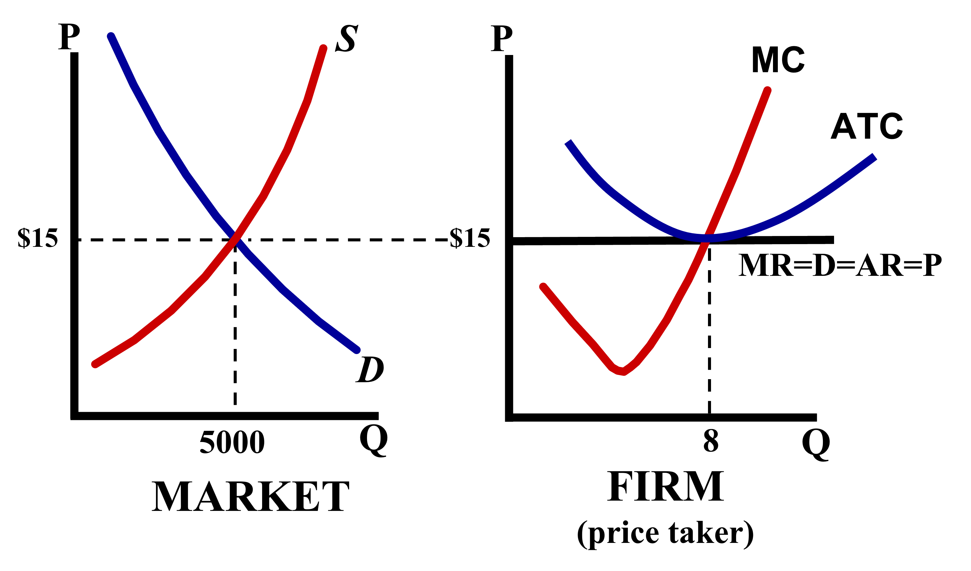

Calcuating the firm's profit using the 3-step process described above will show that the firm makes exactly \(0\) economic profit, and therefore only making a normal profit.